Kibble-Zurek generation of vortex states with finite winding numbers in meshed Kuramoto networks

Theoretical Physics/Engineering PhD project, HES-SO Valais-Wallis

Ongoing

Topic: Assessing robustness and identifying vulnerabilities in deterministically coupled dynamical systems on complex networks

---

Outline

We consider a phase transition, such as Bose-Einstein condensation or superfluid transition. Below the critical temperature, the state is characterized by a macroscopic wavefunction. If one goes through the transition in a thermodynamic way, i.e. infinitely slowly, that wavefunction tends to be constant, with slow amplitude and phase variations.

To generate these topological defects, the Kibble-Zurek mechanism considers going through a phase transition with finite velocity.

The ongoing goal is to explore if such mechanism can be used to generate states with finite winding numbers in meshed Kuramoto networks.

Model and fixed-point solution with different winding numbers

We consider the Kuramoto model

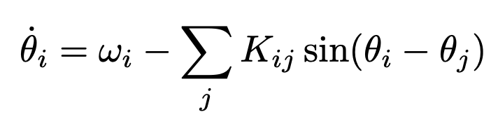
for i = 1, 2, · · · N oscillators, each with its own natural frequency ω_i; when the couplings are numerous and large enough, and for natural frequencies distributed over a finite interval, ω_i ∈ [ω_min > −∞, ω_max < ∞], the system synchronizes in that all oscillators rotate at the same frequency. When the couplings K_ij = ̸= 0 define a meshed network, there may be several synchronous states, differing by integer winding numbers on one or several of the loops formed by the network [1, 2] (s. References below).

How can we generate / reach states with different winding numbers?

Three mechanisms have been identified, when starting from a state with no winding number (q = 0):

• topological changes [3],

• loss of stability of the q = 0 state by parameter variation (coupling strength) [3],

• noise-induced transition [4, 5].

Additionally, to numerically generate a state with given winding number, Ref. [4] developed a method where the dynamics of the Kuramoto model starts from an initially constructed state with given winding number.

These states have finite vorticity, and are therefore similar to vortices in superfluid, i.e. topological defects in a condensate.

The Kibbel-Zurek mechanism generates such topological defects, by going through a phase transition with nonzero velocity.

Procedure:

We start with building a Python code to study the Kuramoto model for identical coupled phase oscillators in order to identify the synchronisation transition point and fixed-point solutions, and then calculate its winding numbers. We define meshed Kuramoto network such as a 2-dimensional hexagonal grid.

---

Some theory background

What is the Kuramoto-Model?

Synchronization is a phenomenon occurring in nature. Some of the most representative examples where synchronisation occurs are flashing fireflies, cheering crowds, metronomes and ticking clocks to clicking present in a large number. Another well-known example where synchronisation of walker's footsteps has lead to unpleasant outcomes was the wobbling of London's Millenium Bridge in 2000.

Steven Strogatz, an applied mathematician best knonw for his work win the areas of nonlinear dynamics and complex system, describes synchronisation as (from his book 'Sync'):

"The tendency to sychronize is one of the most far-reaching drives in all of nature. It extends from people to planets, from animals to atoms. It can be used to describe synchrony in human sleep and circadian rhythms, menstrual synchrony, insect outbreaks, superconductors, lasers, secret codes, heart arrhythmias and fads - a mathematical theme of organisation, or the spontaneous emergence of order out of chaos."

The Kuramoto model, first proposed by Yoshiki Kuramoto, is a mathematical model used to study synchronization behaviour in a wide range of systems described by coupled phase oscillators, where the coupling is assumed to be weak.

The classic Kuramoto model deals with a global (all-to-all) coupling of N periodic oscillators, with with randomly distributed natural frequencies.

By studying the phase dynamics of synchronized (and desynchronized or incoherent) oscillators one can infer the distribution of phases and the order parameter equation (s. later), where a critical coupling strength (usually denoted as K ) determines the occurring of the transition from incoherence to synchronisation of the oscillators. The measure (or degree) of synchrony in the Kuramoto model is defined by the order parameter, which also describes the oscillator's average phase. The order parameter is best understood by considering a unit circle in the complex plane, where the average of the N oscillators, which are represented as points around the unit circle, can be viewed as vectors in the complex plane. If we define the average of the N oscillators (vectors) on the complex plane as z, and the order parameter as r, then r is the absolute value of z, that is r is the magnitude of the average of those vectors, z. When r = 0, there is a minimum, and all phases are scattered around the circle, meaning that the oscillators are incoherent (and they balance each other out). For r = 1, there is maximum, the population of oscillators is in synchrony, and all the phases are identical, which is why the order parameter is often called phase coherence.

If we define the phase of each oscillator's as θ_i, then the following differential equation d(θ_i)/dt defines the interaction of the oscillators.

Each oscillator oscillates at its own natural frequency ω_i (for i = 1,...,N oscillators), that is at a constant angular and the natural frequencies can be seen as distributed over a finite symmetric interval such as a Guassian distribution. K_ij is the coupling parameter of the oscillator i interacting with oscillator j, and for a critical value K_c the oscillators synchronise abruptly (if at all). That is because for each couple of oscillators i and j, if i oscillates ahead of j, i will accelerate j while j will slow down i.

An example of the synchronisation process for an all-to-all model with 20 nodes (oscillators); the vertical blue line defines the critical coupling at which synchronisation occurs :

---

References:

[1] R. Delabays, T. Coletta, and Ph. Jacquod, J. Math. Phys. 57, 032701 (2016). [2] R. Delabays, T. Coletta, and Ph. Jacquod, J. Math. Phys. 58, 032703 (2017). [3] T. Coletta, R. Delabays, I. Adagideli, and Ph. Jacquod, New J. Phys. 18, 103042 (2016). [4] R. Delabays, M. Tyloo, and Ph. Jacquod, Chaos 27, 103109 (2017). [5] M. Tyloo, R. Delabays, and Ph. Jacquod, Phys. Rev. E , 99 062213 (2019).

[6] T.W.B. Kibble, J. Phys. A: Math. Gen. 9, 1387 (1976); Phys. Rep. 67, 183 (1980). [7] W.H. Zurek, Zurek, Nature 317, 505 (1985); Phys. Rep. 276, 177 (1996).

[8] The Kuramoto order parameters https://mathinsight.org/applet/kuramoto_order_parameters

[9] Steven Strogatz, Coupled Oscillators That Synchronize Themselves - Simons Lectures https://www.youtube.com/watch?v=5zFDMyQ8z8g

[10] Ride My Kuramoto Cycle - Synchronization of Phase-Coupled Oscillators https://www.complexity-explorables.org/explorables/ride-my-kuramotocycle/

[11] From Kuramoto to Crawford: exploring the onset of synchronization in populations of coupled oscillators https://static.squarespace.com/static/5436e695e4b07f1e91b30155/t/544525a8e4b0b8e2e8230fa3/1413817768995/from-kuramoto-to-crawford.pdf